3 Asymptotics
3.1 Introduction
In the last chapter, we defined estimators and started investigating their finite-sample properties like unbiasedness and the sampling variance. We call these “finite-sample” properties since they hold at any sample size. We saw that under iid data, the sample mean is unbiased for the population mean, but this result holds as much for \(n = 10\) as it does for \(n = 1,000,000\). But these properties are also of limited use: we only learn the center and spread of the sampling distribution of \(\Xbar_n\) from these results. What about the shape of the distribution? We can often derive the shape if we are willing to make certain assumptions on the underlying data (for example, if the data is normal, then the sample means will also be normal). Still, this approach is brittle: if our parametric assumption is false, we’re back to square one.
In this chapter, we will take a different approach and see what happens to the sampling distribution of estimators as the sample size gets large, which we refer to as asymptotic theory. While asymptotics will often simplify our derivations, it is essential to understand everything we do with asymptotics will be an approximation. No one ever has infinite data, but we hope that the approximations will be closer to the truth as our samples get larger.
3.2 Why convergence with probability is hard
It’s helpful to review the basic idea of convergence in deterministic sequences from calculus:
Definition 3.1 A sequence \(\{a_n: n = 1, 2, \ldots\}\) has the limit \(a\) written \(a_n \rightarrow a\) as \(n\rightarrow \infty\) or \(\lim_{n\rightarrow \infty} a_n = a\) if for all \(\epsilon > 0\) there is some \(n_{\epsilon} < \infty\) such that for all \(n \geq n_{\epsilon}\), \(|a_n - a| \leq \epsilon\).
We say that \(a_n\) converges to \(a\) if \(\lim_{n\rightarrow\infty} a_n = a\). Basically, a sequence converges to a number if the sequence gets closer and closer to that number as the sequence goes on.
Can we apply this same idea to sequences of random variables (like estimators)? Let’s look at a few examples that help clarify why this might be difficult.1 Let’s say that we have a sequence of \(a_n = a\) for all \(n\) (that is, a constant sequence). Then obviously \(\lim_{n\rightarrow\infty} a_n = a\). Now let’s say we have a sequence of random variables, \(X_1, X_2, \ldots\), that are all independent with a standard normal distribution, \(N(0,1)\). From the analogy to the deterministic case, it is tempting to say that \(X_n\) converges to \(X \sim N(0, 1)\), but notice that because they are all different random variables, \(\P(X_n = X) = 0\). Thus, we must be careful about saying how one variable converges to another variable.
Another example highlights subtle problems with a sequence of random variables converging to a single value. Suppose we have a sequence of random variables \(X_1, X_2, \ldots\) where \(X_n \sim N(0, 1/n)\). Clearly, the distribution of \(X_n\) will concentrate around 0 for large values of \(n\), so it is tempting to say that \(X_n\) converges to 0. But notice that \(\P(X_n = 0) = 0\) because of the nature of continuous random variables.
3.3 Convergence in probability and consistency
There are several different ways that a sequence of random variance can converge. The first type of convergence deals with sequences converging to a single value.2
Definition 3.2 A sequence of random variables, \(X_1, X_2, \ldots\), is said to converge in probability to a value \(b\) if for every \(\varepsilon > 0\), \[ \P(|X_n - b| > \varepsilon) \rightarrow 0, \] as \(n\rightarrow \infty\). We write this \(X_n \inprob b\).
With deterministic sequences, we said that \(a_n\) converges to \(a\) as it gets closer and closer to \(a\) as \(n\) gets bigger. For convergence in probability, the sequence of random variables converges to \(b\) if the probability that random variables are far away from \(b\) gets smaller and smaller as \(n\) gets big.
Notation alert
You will sometimes see convergence in probability written as \(\text{plim}(Z_n) = b\) if \(Z_n \inprob b\), \(\text{plim}\) stands for “probability limit.”
Convergence in probability is crucial for evaluating estimators. While we said that unbiasedness was not the be-all and end-all of properties of estimators, the following property is an essential and fundamental property that we would like all good estimators to have.
Definition 3.3 An estimator is consistent if \(\widehat{\theta}_n \inprob \theta\).
Consistency of an estimator implies that the sampling distribution of this estimator “collapses” on the true value as the sample size gets large. We say an estimator is inconsistent if it converges in probability to any other value, which is obviously a terrible property of an estimator. As the sample size gets large, the probability that an inconsistent estimator will be close to the truth will approach 0.
We can also define convergence in probability for a sequence of random vectors, \(\X_1, \X_2, \ldots\), where \(\X_i = (X_{i1}, \ldots, X_{ik})\) is a random vector of length \(k\). This sequence convergences in probability to a vector \(\mb{b} = (b_1, \ldots, b_k)\) if and only if each random variable in the vector converges to the corresponding element in \(\mb{b}\), or that \(X_{nj} \inprob b_j\) for all \(j = 1, \ldots, k\).
3.4 Useful inequalities
At first glance, establishing an estimator’s consistency will be difficult. How can we know if a distribution will collapse to a specific value without knowing the shape or family of the distribution? It turns out that there are certain relationships between the mean and variance of a random variable and certain probability statements that hold for all distributions (that have finite variance, at least). These relationships will be crucial to establishing results that do not depend on a specific distribution.
Theorem 3.1 (Markov Inequality) For any r.v. \(X\) and any \(\delta >0\), \[ \P(|X| \geq \delta) \leq \frac{\E[|X|]}{\delta}. \]
Proof. Notice that we can let \(Y = |X|/\delta\) and rewrite the statement as \(\P(Y \geq 1) \leq \E[Y]\) (since \(\E[|X|]/\delta = \E[|X|/\delta]\) by the properties of expectation), which is what we will show. But notice that \[ \mathbb{I}(Y \geq 1) \leq Y. \] Why does this hold? We can investigate the two possible values of the indicator function to see. If \(Y\) is less than 1, then the indicator function will be 0, but recall that \(Y\) is nonnegative, so we know that it must be at least as big as 0 so that inequality holds. If \(Y \geq 1\), then the indicator function will take the value one, but we just said that \(Y \geq 1\), so the inequality holds. If we take the expectation of both sides of this inequality, we obtain the result (remember, the expectation of an indicator function is the probability of the event).
In words, Markov’s inequality says that the probability of a random variable being large in magnitude cannot be high if the average is not large in magnitude. Blitzstein and Hwang (2019) provide an excellent intuition behind this result. Let \(X\) be the income of a randomly selected individual in a population and set \(\delta = 2\E[X]\) so that the inequality becomes \(\P(X > 2\E[X]) < 1/2\) (assuming that all income is nonnegative). Here, the inequality says that the share of the population with an income twice the average must be less than 0.5 since if more than half the population were making twice the average income, then the average would have to be higher.
It’s pretty astounding how general this result is since it holds for all random variables. Of course, its generality comes at the expense of not being very informative. If \(\E[|X|] = 5\), for instance, the inequality tells us that \(\P(|X| \geq 1) \leq 5\), which is not very helpful since we already know that probabilities are less than 1! We can get tighter bounds if we are willing to make some assumptions about \(X\).
Theorem 3.2 (Chebyshev Inequality) Suppose that \(X\) is r.v. for which \(\V[X] < \infty\). Then, for every real number \(\delta > 0\), \[ \P(|X-\E[X]| \geq \delta) \leq \frac{\V[X]}{\delta^2}. \]
Proof. To prove this, we only need to square both sides of the inequality inside the probability statement and apply Markov’s inequality: \[ \P\left( |X - \E[X]| \geq \delta \right) = \P((X-\E[X])^2 \geq \delta^2) \leq \frac{\E[(X - \E[X])^2]}{\delta^2} = \frac{\V[X]}{\delta^2}, \] with the last equality holding by the definition of variance.
Chebyshev’s inequality is a straightforward extension of the Markov result: the probability of a random variable being far from its mean (that is, \(|X-\E[X]|\) being large) is limited by the variance of the random variable. If we let \(\delta = c\sigma\), where \(\sigma\) is the standard deviation of \(X\), then we can use this result to bound the normalized: \[ \P\left(\frac{|X - \E[X]|}{\sigma} > c \right) \leq \frac{1}{c^2}. \] This statement says the probability of being two standard deviations away from the mean must be less than 1/4 = 0.25. Notice that this bound can be fairly wide. If \(X\) has a normal distribution, we know that about 5% of draws will be greater than 2 SDs away from the mean, much lower than the 25% bound implied by Chebyshev’s inequality.
3.5 The law of large numbers
We can now use these inequalities to show how estimators can be consistent for their target quantities of interest. Why are these inequalities helpful for this purpose? Remember that convergence in probability was about the probability of an estimator being far away from a value going to zero. Chebyshev’s inequality shows that we can bound these exact probabilities.
The most famous consistency result has a special name.
Theorem 3.3 (Weak Law of Large Numbers) Let \(X_1, \ldots, X_n\) be i.i.d. draws from a distribution with mean \(\mu = \E[X_i]\) and variance \(\sigma^2 = \V[X_i] < \infty\). Let \(\Xbar_n = \frac{1}{n} \sum_{i =1}^n X_i\). Then, \(\Xbar_n \inprob \mu\).
Proof. Recall that the sample mean is unbiased, so \(\E[\Xbar_n] = \mu\) with sampling variance \(\sigma^2/n\). We can then apply Chebyshev to the sample mean to get \[ \P(|\Xbar_n - \mu| \geq \delta) \leq \frac{\sigma^2}{n\delta^2} \] An \(n\rightarrow\infty\), the right-hand side goes to 0, which means that the left-hand side also must go to 0, which is the definition of \(\Xbar_n\) converging in probability to \(\mu\).
The weak law of large numbers (WLLN) shows that, under general conditions, the sample mean gets closer to the population mean as \(n\rightarrow\infty\). This result holds even when the variance of the data is infinite, though that’s a situation that most analysts will rarely face.
Note
The naming of the “weak” law of large numbers seems to imply the existence of a “strong” law of large numbers (SLLN), and this is true. The SLLN states that the sample mean converges to the population mean with probability 1. This type of convergence, called almost sure convergence, is stronger than convergence in probability which only says that the probability of the sample mean being close to the population mean converges to 1. While it is nice to know that this stronger form of convergence holds for the sample mean under the same assumptions, it is rare for folks outside of theoretical probability and statistics to rely on almost sure convergence.
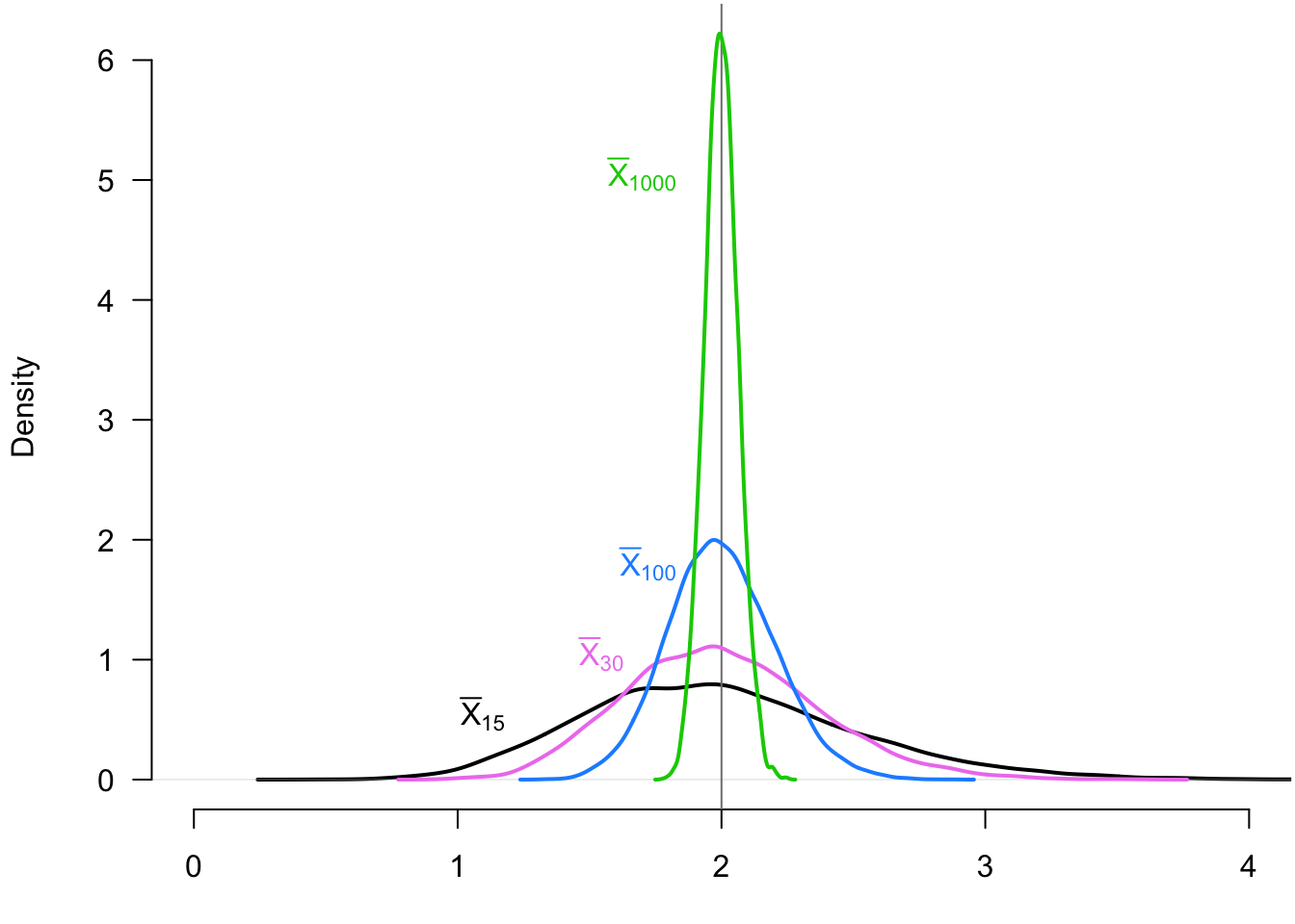
Example 3.1 It can be helpful to see how the distribution of the sample mean changes as a function of the sample size to appreciate the WLLN. We can show this by taking repeated iid samples of different sizes from an exponential random variable with rate parameter 0.5 so that \(\E[X_i] = 2\). In Figure 3.1, we show the distribution of the sample mean (across repeated samples) when the sample size is 15 (black), 30 (violet), 100 (blue), and 1000 (green). We can see how the sample mean distribution is “collapsing” on the true population mean, 2. The probability of being far away from 2 becomes progressively smaller.
The WLLN also holds for random vectors in addition to random variables. Let \((\X_1, \ldots, \X_n)\) be an iid sample of random vectors of length \(k\), \(\mb{X}_i = (X_{i1}, \ldots, X_{ik})\). We can define the vector sample mean as just the vector of sample means for each of the entries:
\[ \overline{\mb{X}}_n = \frac{1}{n} \sum_{i=1}^n \mb{X}_i = \begin{pmatrix} \Xbar_{n,1} \\ \Xbar_{n,2} \\ \vdots \\ \Xbar_{n, k} \end{pmatrix} \] Since this is just a vector of sample means, each random variable in the random vector will converge in probability to the mean of that random variable. Fortunately, this is the exact definition of convergence in probability for random vectors. We formally write this in the following theorem.
Theorem 3.4 If \(\X_i \in \mathbb{R}^k\) are iid draws from a distribution with \(\E[X_{ij}] < \infty\) for all \(j=1,\ldots,k\) then as \(n\rightarrow\infty\)
\[ \overline{\mb{X}}_n \inprob \E[\X] = \begin{pmatrix} \E[X_{i1}] \\ \E[X_{i2}] \\ \vdots \\ \E[X_{ik}] \end{pmatrix}. \]
Notation alert
You will have noticed that many of the formal results we have presented so far have “moment conditions” that certain moments are finite. For the vector WLLN, we saw that applied to the mean of each variable in the vector. Some books use a shorthand for this: \(\E\Vert \X_i\Vert < \infty\), where \[ \Vert\X_i\Vert = \left(X_{i1}^2 + X_{i2}^2 + \ldots + X_{ik}^2\right)^{1/2}. \] This expression has slightly more compact notation, but why does it work? One can show that this function, called the Euclidean norm or \(L_2\)-norm, is a convex function, so we can apply Jensen’s inequality to show that: \[ \E\Vert \X_i\Vert \geq \Vert \E[\X_i] \Vert = (\E[X_{i1}]^2 + \ldots + \E[X_{ik}]^2)^{1/2}. \] So if \(\E\Vert \X_i\Vert\) is finite, all the component means are finite. Otherwise, the right-hand side of the previous equation would be infinite.
3.6 Consistency of estimators
The WLLN shows that the sample mean of iid draws is consistent for the population mean, which is a massive result given that so many estimators are sample means of potentially complicated functions of the data. What about other estimators? The proof of the WLLN points to one way to determine if an estimator is consistent: if it is unbiased and the sampling variance shrinks as the sample size grows.
Theorem 3.5 For any estimator \(\widehat{\theta}_n\), if \(\text{bias}[\widehat{\theta}_n] = 0\) and \(\V[\widehat{\theta}_n] \rightarrow 0\) as \(n\rightarrow \infty\), then \(\widehat{\theta}_n\) is consistent.
Thus, for unbiased estimators, if we can characterize its sampling variance, we should be able to tell if it is consistent. This result is handy since working with the probability statements used for the WLLN can sometimes be quite confusing.
What about biased estimators? Consider a plug-in estimator like \(\widehat{\alpha} = \log(\Xbar_n)\) where \(X_1, \ldots, X_n\) are iid from a population with mean \(\mu\). We know that for nonlinear functions like logarithms we have \(\log\left(\E[Z]\right) \neq \E[\log(Z)]\), so \(\E[\widehat{\alpha}] \neq \log(\E[\Xbar_n])\) and the plug-in estimator will be biased for \(\log(\mu)\). It will also be difficult to obtain an expression for the bias in terms of \(n\). Is all hope lost here? Must we give up on consistency? No, and in fact, consistency will be much simpler to show in this setting.
Theorem 3.6 (Properties of convergence in probability) Let \(X_n\) and \(Z_n\) be two sequences of random variables such that \(X_n \inprob a\) and \(Z_n \inprob b\), and let \(g(\cdot)\) be a continuous function. Then,
- \(g(X_n) \inprob g(a)\) (continuous mapping theorem)
- \(X_n + Z_n \inprob a + b\)
- \(X_nZ_n \inprob ab\)
- \(X_n/Z_n \inprob a/b\) if \(b > 0\).
We can now see that many of the nasty problems with expectations and nonlinear functions are made considerably easier with convergence in probability in the asymptotic setting. So while we know that \(\log(\Xbar_n)\) is biased for \(\log(\mu)\), we know that it is consistent since \(\log(\Xbar_n) \inprob \log(\mu)\) because \(\log\) is a continuous function.
Example 3.2 Suppose we implemented a survey by randomly selecting a sample from the population of size \(n\), but not everyone responded to our survey. Let the data consist of pairs of random variables, \((Y_1, R_1), \ldots, (Y_n, R_n)\), where \(Y_i\) is the question of interest and \(R_i\) is a binary indicator for if the respondent answered the question (\(R_i = 1\)) or not (\(R_i = 0\)). Our goal is to estimate the mean of the question for responders: \(\E[Y_i \mid R_i = 1]\). We can use the law of iterated expectation to obtain \[ \begin{aligned} \E[Y_iR_i] &= \E[Y_i \mid R_i = 1]\P(R_i = 1) + \E[ 0 \mid R_i = 0]\P(R_i = 0) \\ \implies \E[Y_i \mid R_i = 1] &= \frac{\E[Y_iR_i]}{\P(R_i = 1)} \end{aligned} \]
The relevant estimator for this quantity is the mean of the outcome among those who responded, which is slightly more complicated than a typical sample mean because the denominator is a random variable: \[ \widehat{\theta}_n = \frac{\sum_{i=1}^n Y_iR_i}{\sum_{i=1}^n R_i}. \] Notice that this estimator is the ratio of two random variables. The numerator has mean \(n\E[Y_iR_i]\) and the denominator has mean \(n\P(R_i = 1)\). It is then tempting to say that we can take the ratio of these means as the mean of \(\widehat{\theta}_n\), but expectations are not preserved in nonlinear functions like this.
We can establish consistency of our estimator, though, by noting that we can rewrite the estimator as a ratio of sample means \[ \widehat{\theta}_n = \frac{(1/n)\sum_{i=1}^n Y_iR_i}{(1/n)\sum_{i=1}^n R_i}, \] where by the WLLN the numerator \((1/n)\sum_{i=1}^n Y_iR_i \inprob \E[Y_iR_i]\) and the denominator \((1/n)\sum_{i=1}^n R_i \inprob \P(R_i = 1)\). Thus, by Theorem 3.6, we have \[ \widehat{\theta}_n = \frac{(1/n)\sum_{i=1}^n Y_iR_i}{(1/n)\sum_{i=1}^n R_i} \inprob \frac{\E[Y_iR_i]}{\P[R_i = 1]} = \E[Y_i \mid R_i = 1], \] so long as the probability of responding is greater than zero. This establishes that our sample mean among responders, while biased for the conditional expectation among responders, is consistent for that quantity.
Keeping the difference between unbiased and consistent clear in your mind is essential. You can easily create ridiculous unbiased estimators that are inconsistent. Let’s return to our iid sample, \(X_1, \ldots, X_n\), from a population with \(E[X_i] = \mu\). There is nothing in the rule book against defining an estimator \(\widehat{\theta}_{first} = X_1\) that uses the first observation as the estimate. This estimator is silly, but it is unbiased since \(\E[\widehat{\theta}_{first}] = \E[X_1] = \mu\). It is inconsistent since the sampling variance of this estimator is just the variance of the population distribution, \(\V[\widehat{\theta}_{first}] = \V[X_i] = \sigma^2\), which does not change as a function of the sample size. Generally speaking, we can regard “unbiased but inconsistent” estimators as silly and not worth our time (along with biased and inconsistent estimators).
Some estimators are biased but consistent that are often much more interesting. We already saw one such estimator in Example 3.2, but there are many more. Maximum likelihood estimators, for example, are (under some regularity conditions) consistent for the parameters of a parametric model but are often biased.
To study these estimator, we can broaden Theorem 3.5 to the class of asymptotically unbiased estimators that have bias that vanishes as the sample size grows.
Theorem 3.7 For any estimator \(\widehat{\theta}_n\), if \(\text{bias}[\widehat{\theta}_n] \to 0\) and \(\V[\widehat{\theta}_n] \rightarrow 0\) as \(n\rightarrow \infty\), then \(\widehat{\theta}_n\) is consistent.
Example 3.3 (Plug-in variance estimator) In the last chapter, we introduced the plug-in estimator for the population variance, \[ \widehat{\sigma}^2 = \frac{1}{n} \sum_{i=1}^n (X_i - \Xbar_n)^2, \] which we will now show is biased but consistent. To see the bias note that we can rewrite the sum of square deviations \[\sum_{i=1}^n (X_i - \Xbar_n)^2 = \sum_{i=1}^n X_i^2 - n\Xbar_n^2. \] Then, the expectation of the plug-in estimator is \[ \begin{aligned} \E[\widehat{\sigma}^2] & = \E\left[\frac{1}{n}\sum_{i=1}^n X_i^2\right] - \E[\Xbar_n^2] \\ &= \E[X_i^2] - \frac{1}{n^2}\sum_{i=1}^n \sum_{j=1}^n \E[X_iX_j] \\ &= \E[X_i^2] - \frac{1}{n^2}\sum_{i=1}^n \E[X_i^2] - \frac{1}{n^2}\sum_{i=1}^n \sum_{j\neq i} \underbrace{\E[X_i]\E[X_j]}_{\text{independence}} \\ &= \E[X_i^2] - \frac{1}{n}\E[X_i^2] - \frac{1}{n^2} n(n-1)\mu^2 \\ &= \frac{n-1}{n} \left(\E[X_i^2] - \mu^2\right) \\ &= \frac{n-1}{n} \sigma^2 = \sigma^2 - \frac{1}{n}\sigma^2 \end{aligned}. \] Thus, we can see that the bias of the plug-in estimator is \(-(1/n)\sigma^2\), so it slightly underestimates the variance. Nicely, though, the bias shrinks as a function of the sample size, so according to Theorem 3.7, it will be consistent so long as the sampling variance of \(\widehat{\sigma}^2\) shrinks as a function of the sample size, which it does (though omit that proof here). Of course, simply multiplying this estimator by \(n/(n-1)\) will give an unbiased and consistent estimator that is also the typical sample variance estimator.
3.7 Convergence in distribution and the central limit theorem
Convergence in probability and the law of large numbers are beneficial for understanding how our estimators will (or will not) collapse to their estimand as the sample size increases. But what about the shape of the sampling distribution of our estimators? For statistical inference, we would like to be able to make probability statements such as \(\P(a \leq \widehat{\theta}_n \leq b)\). These statements will be the basis of hypothesis testing and confidence intervals. But to make those types of statements, we need to know the entire distribution of \(\widehat{\theta}_n\), not just the mean and variance. Luckily, established results will allow us to approximate the sampling distribution of a vast swath of estimators when our sample sizes are large.
We need first to describe a weaker form of convergence to see how we will develop these approximations.
Definition 3.4 Let \(X_1,X_2,\ldots\), be a sequence of r.v.s, and for \(n = 1,2, \ldots\) let \(F_n(x)\) be the c.d.f. of \(X_n\). Then it is said that \(X_1, X_2, \ldots\) converges in distribution to r.v. \(X\) with c.d.f. \(F(x)\) if \[ \lim_{n\rightarrow \infty} F_n(x) = F(x), \] for all values of \(x\) for which \(F(x)\) is continuous. We write this as \(X_n \indist X\) or sometimes \(X_n ⇝ X\).
Essentially, convergence in distribution means that as \(n\) gets large, the distribution of \(X_n\) becomes more and more similar to the distribution of \(X\), which we often call the asymptotic distribution of \(X_n\) (other names include the large-sample distribution). If we know that \(X_n \indist X\), then we can use the distribution of \(X\) as an approximation to the distribution of \(X_n\), and that distribution can be reasonably accurate.
One of the most remarkable results in probability and statistics is that a large class of estimators will converge in distribution to one particular family of distributions: the normal. This result is one reason we study the normal so much and why investing in building intuition about it will pay off across many domains of applied work. We call this broad class of results the “central limit theorem” (CLT), but it would probably be more accurate to refer to them as “central limit theorems” since much of statistics is devoted to showing the result in different settings. We now present the simplest CLT for the sample mean.
Theorem 3.8 (Central Limit Theorem) Let \(X_1, \ldots, X_n\) be i.i.d. r.v.s from a distribution with mean \(\mu = \E[X_i]\) and variance \(\sigma^2 = \V[X_i]\). Then if \(\E[X_i^2] < \infty\), we have \[ \frac{\Xbar_n - \mu}{\sqrt{\V[\Xbar_n]}} = \frac{\sqrt{n}\left(\Xbar_n - \mu\right)}{\sigma} \indist \N(0, 1). \]
In words: the sample mean of a random sample from a population with finite mean and variance will be approximately normally distributed in large samples. Notice how we have not made any assumptions about the distribution of the underlying random variables, \(X_i\). They could be binary, event count, continuous, or anything. The CLT is incredibly broadly applicable.
Notation alert
Why do we state the CLT in terms of the sample mean after centering and scaling by its standard error? Suppose we don’t normalize the sample mean in this way. In that case, it isn’t easy to talk about convergence in distribution because we know from the WLLN that \(\Xbar_n \inprob \mu\), so in the limit, the distribution of \(\Xbar_n\) is concentrated at point mass around that value. Normalizing by centering and rescaling ensures that the variance of the resulting quantity will not depend on \(n\), so it makes sense to talk about its distribution converging. Sometimes you will see the equivalent result as \[ \sqrt{n}\left(\Xbar_n - \mu\right) \indist \N(0, \sigma^2). \]
We can use this result to state approximations that we can use when discussing estimators such as \[ \Xbar_n \overset{a}{\sim} N(\mu, \sigma^2/n), \] where we use \(\overset{a}{\sim}\) to be “approximately distributed as in large samples.” This approximation allows us to say things like: “in large samples, we should expect the sample mean to between within \(2\sigma/\sqrt{n}\) of the true mean in 95% of repeated samples.” These statements will be essential for hypothesis tests and confidence intervals! Estimators so often follow the CLT that we have an expression for this property.
Definition 3.5 An estimator \(\widehat{\theta}_n\) is asymptotically normal if for some \(\theta\) \[ \sqrt{n}\left( \widehat{\theta}_n - \theta \right) \indist N\left(0,\V_{\theta}\right). \]
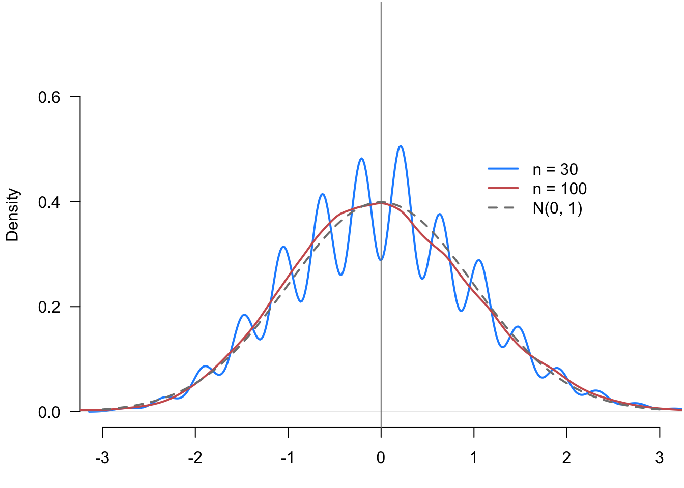
Example 3.4 To illustrate how the CLT works, we can simulate the sampling distribution of the (normalized) sample mean at different sample sizes. Let \(X_1, \ldots, X_n\) be iid samples from a Bernoulli with probability of success 0.25. We then draw repeated samples of size \(n=30\) and \(n=100\) and calculate \(\sqrt{n}(\Xbar_n - 0.25)/\sigma\) for each random sample. Figure 3.2 plots the density of these two sampling distributions along with a standard normal reference. We can see that even at \(n=30\), the rough shape of the density looks normal, with spikes and valleys due to the discrete nature of the data (the sample mean can only take on 31 possible values in this case). By \(n=100\), the sampling distribution is very close to the true standard normal.
There are several properties of convergence in distribution that are helpful to us.
Theorem 3.9 (Properties of convergence in distribution) Let \(X_n\) be a sequence of random variables \(X_1, X_2,\ldots\) that converges in distribution to some rv \(X\) and let \(Y_n\) be a sequence of random variables \(Y_1, Y_2,\ldots\) that converges in probability to some number, \(c\). Then,
- \(g(X_n) \indist g(X)\) for all continuous functions \(g\).
- \(X_nY_n\) converges in distribution to \(cX\)
- \(X_n + Y_n\) converges in distribution to \(X + c\)
- \(X_n / Y_n\) converges in distribution to \(X / c\) if \(c \neq 0\)
We refer to the last three results as Slutsky’s theorem. These results are often crucial for determining an estimator’s asymptotic distribution.
A critical application of Slutsky’s theorem is when we replace the (unknown) population variance in the CLT with an estimate. Recall the definition of the sample variance as \[ S_n^2 = \frac{1}{n-1} \sum_{i=1}^n (X_i - \Xbar_n)^2, \] with the sample standard deviation defined as \(S_{n} = \sqrt{S_{n}^2}\). It’s easy to show that these are consistent estimators for their respective population parameters \[ S_{n}^2 \inprob \sigma^2 = \V[X_i], \qquad S_{n} \inprob \sigma, \] which, by Slutsky’s theorem, implies that \[ \frac{\sqrt{n}\left(\Xbar_n - \mu\right)}{S_n} \indist \N(0, 1) \] Comparing this result to the statement of CLT, we see that replacing the population variance with a consistent estimate of the variance (or standard deviation) does not affect the asymptotic distribution.
Like with the WLLN, the CLT holds for random vectors of sample means, where their centered and scaled versions converge to a multivariate normal distribution with a covariance matrix equal to the covariance matrix of the underlying random vectors of data, \(\X_i\).
Theorem 3.10 If \(\mb{X}_i \in \mathbb{R}^k\) are i.i.d. and \(\E\Vert \mb{X}_i \Vert^2 < \infty\), then as \(n \to \infty\), \[ \sqrt{n}\left( \overline{\mb{X}}_n - \mb{\mu}\right) \indist \N(0, \mb{\Sigma}), \] where \(\mb{\mu} = \E[\mb{X}_i]\) and \(\mb{\Sigma} = \V[\mb{X}_i] = \E\left[(\mb{X}_i-\mb{\mu})(\mb{X}_i - \mb{\mu})'\right]\).
Notice that \(\mb{\mu}\) is the vector of population means for all the random variables in \(\X_i\) and \(\mb{\Sigma}\) is the variance-covariance matrix for that vector.
Note
As with the notation alert with the WLLN, we are using shorthand here, \(\E\Vert \mb{X}_i \Vert^2 < \infty\), which implies that \(\E[X_{ij}^2] < \infty\) for all \(j = 1,\ldots, k\), or equivalently, that the variances of each variable in the sample means has finite variance.
3.8 Confidence intervals
We now turn to an essential application of the central limit theorem: confidence intervals.
You have run your experiment and presented your readers with your single best guess about the treatment effect with the difference in sample means. You may have also presented the estimated standard error of this estimate to give readers a sense of how variable the estimate is. But none of these approaches answer a fairly compelling question: what range of values of the treatment effect is plausible given the data we observe?
A point estimate typically has 0 probability of being the exact true value, but intuitively we hope that the true value is close to this estimate. Confidence intervals make this kind of intuition more formal by instead estimating ranges of values with a fixed percentage of these ranges containing the actual parameter value.
We begin with the basic definition of a confidence interval.
Definition 3.6 A \(1-\alpha\) confidence interval for a real-valued parameter \(\theta\) is a pair of statistics \(L= L(X_1, \ldots, X_n)\) and \(U = U(X_1, \ldots, X_n)\) such that \(L < U\) for all values of the sample and such that \[ \P(L \leq \theta \leq U \mid \theta) \geq 1-\alpha, \quad \forall \theta \in \Theta. \]
We say that a \(1-\alpha\) confidence interval covers (contains, captures, traps, etc.) the true value at least \(100(1-\alpha)\%\) of the time, and we refer to \(1-\alpha\) as the coverage probability or simply coverage. Typical confidence intervals include 95% percent (\(\alpha = 0.05\)) and 90% (\(\alpha = 0.1\)).
So a confidence interval is a random interval with a particular guarantee about how often it will contain the true value. It’s important to remember what is random and what is fixed in this setup. The interval varies from sample to sample, but the true value of the parameter stays fixed, and the coverage is how often we should expect the interval to contain that true value. The “repeating my sample over and over again” analogy can break down very quickly, so it’s sometimes helpful to interpret it as giving guarantees across confidence intervals across different experiments. In particular, suppose that a journal publishes 100 quantitative articles annually, each producing a single 95% confidence interval for their quantity of interest. Then, if the confidence intervals are valid, we should expect 95 of those confidence intervals to contain the true value.
Warning
Suppose you calculate a 95% confidence interval, \([0.1, 0.4]\). It’s tempting to make a probability statement like \(\P(0.1 \leq \theta \leq 0.4 \mid \theta) = 0.95\) or that there’s a 95% chance that the parameter is in \([0.1, 0.4]\). But looking at the probability statement, everything on the left-hand side of the conditioning bar is fixed, so the probability either has to be 0 (\(\theta\) is outside the interval) or 1 (\(\theta\) is in the interval). The coverage probability of a confidence interval refers to its status as a pair of random variables, \((L, U)\), not any particular realization of those variables like \((0.1, 0.4)\). As an analogy, consider if calculated the sample mean as \(0.25\) and then try to say that \(0.25\) is unbiased for the population mean. This statement doesn’t make sense because unbiasedness refers to how the sample mean varies from sample to sample.
In most cases, we will not be able to derive exact confidence intervals but rather confidence intervals that are asymptotically valid, which means that if we write the interval as a function of the sample size, \((L_n, U_n)\), they would have asymptotic coverage \[ \lim_{n\to\infty} \P(L_n \leq \theta \leq U_n) \geq 1-\alpha \quad\forall\theta\in\Theta. \]
Asymptotic coverage is the property we can show for most confidence intervals since we usually rely on large sample approximations based on the central limit theorem.
3.8.1 Deriving confidence intervals
If you have taken any statistics before, you probably have seen the standard formula for the 95% confidence interval of the sample mean, \[ \left[\Xbar_n - 1.96\frac{s}{\sqrt{n}},\; \Xbar_n + 1.96\frac{s}{\sqrt{n}}\right], \] where you can recall that \(s\) is the sample standard deviation and \(s/\sqrt{n}\) is the estimate of the standard error of the sample mean. If this is a 95% confidence interval, then the probability that it contains the population mean \(\mu\) should be 0.95, but how can we derive this? We can justify this logic using the central limit theorem, and the argument will hold for any asymptotically normal estimator.
Let’s say that we have an estimator, \(\widehat{\theta}_n\) for the parameter \(\theta\) with estimated standard error \(\widehat{\se}[\widehat{\theta}_n]\). If the estimator is asymptotically normal, then in large samples, we know that \[ \frac{\widehat{\theta}_n - \theta}{\widehat{\se}[\widehat{\theta}_n]} \sim \N(0, 1). \] We can then use our knowledge of the standard normal and the empirical rule to find \[ \P\left( -1.96 \leq \frac{\widehat{\theta}_n - \theta}{\widehat{\se}[\widehat{\theta}_n]} \leq 1.96\right) = 0.95 \] and by multiplying each part of the inequality by \(\widehat{\se}[\widehat{\theta}_n]\), we get \[ \P\left( -1.96\,\widehat{\se}[\widehat{\theta}_n] \leq \widehat{\theta}_n - \theta \leq 1.96\,\widehat{\se}[\widehat{\theta}_n]\right) = 0.95, \] We then subtract all parts by the estimator to get \[ \P\left(-\widehat{\theta}_n - 1.96\,\widehat{\se}[\widehat{\theta}_n] \leq - \theta \leq -\widehat{\theta}_n + 1.96\,\widehat{\se}[\widehat{\theta}_n]\right) = 0.95, \] and finally we multiply all parts by \(-1\) (and flipping the inequalities) to arrive at \[ \P\left(\widehat{\theta}_n - 1.96\,\widehat{\se}[\widehat{\theta}_n] \leq \theta \leq \widehat{\theta}_n + 1.96\,\widehat{\se}[\widehat{\theta}_n]\right) = 0.95. \] To connect back to the definition of the confidence interval, we have now shown that the random interval \([L, U]\) where \[ \begin{aligned} L = L(X_1, \ldots, X_n) &= \widehat{\theta}_n - 1.96\,\widehat{\se}[\widehat{\theta}_n] \\ U = U(X_1, \ldots, X_n) &= \widehat{\theta}_n + 1.96\,\widehat{\se}[\widehat{\theta}_n], \end{aligned} \] is an asymptotically valid estimator.3 Replacing \(\Xbar_n\) for \(\widehat{\theta}_n\) and \(s/\sqrt{n}\) for \(\widehat{\se}[\widehat{\theta}_n]\) establishes how the standard 95% confidence interval for the sample mean above is asymptotically valid.
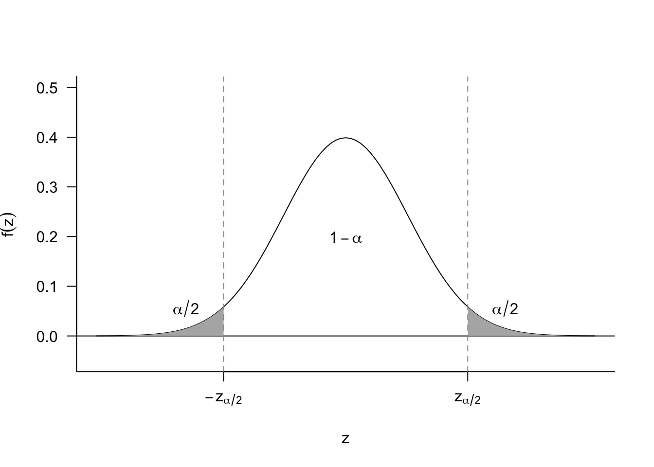
How can we generalize this to \(1-\alpha\) confidence intervals? For a standard normal rv, \(Z\), we know that \[ \P(-z_{\alpha/2} \leq Z \leq z_{\alpha/2}) = 1-\alpha \] which implies that we can obtain a \(1-\alpha\) asymptotic confidence intervals by using the interval \([L, U]\), where \[ L = \widehat{\theta}_{n} - z_{\alpha/2} \widehat{\se}[\widehat{\theta}_{n}], \quad U = \widehat{\theta}_{n} + z_{\alpha/2} \widehat{\se}[\widehat{\theta}_{n}]. \] This is sometimes shortened to \(\widehat{\theta}_n \pm z_{\alpha/2} \widehat{\se}[\widehat{\theta}_{n}]\). Remember that we can obtain the values of \(z_{\alpha/2}\) easily from R:
## alpha = 0.1 for 90% CI
qnorm(0.1 / 2, lower.tail = FALSE)
[1] 1.644854As a concrete example, then, we could derive a 90% asymptotic confidence interval for the sample mean as \[ \left[\Xbar_{n} - 1.64 \frac{\widehat{\sigma}}{\sqrt{n}}, \Xbar_{n} + 1.64 \frac{\widehat{\sigma}}{\sqrt{n}}\right] \]
3.8.2 Interpreting confidence intervals
Remember that the interpretation of confidence is how the random interval performs over repeated samples. A valid 95% confidence interval is a random interval containing the true value in 95% of samples. Simulating repeated samples helps clarify this.
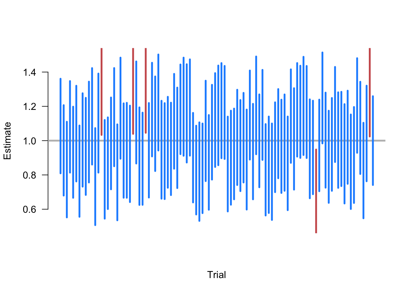
Example 3.5 Suppose we are taking samples of size \(n=500\) of random variables where \(X_i \sim \N(1, 10)\), and we want to estimate the population mean \(\E[X] = 1\). To do so, we repeat the following steps:
- Draw a sample of \(n=500\) from \(\N(1, 10)\).
- Calculate the 95% confidence interval sample mean \(\Xbar_n \pm 1.96\widehat{\sigma}/\sqrt{n}\).
- Plot the intervals along the x-axis and color them blue if they contain the truth (1) and red if not.
Figure 3.4 shows 100 iterations of these steps. We see that, as expected, most calculated CIs contain the true value. Five random samples produce intervals that fail to include 1, an exact coverage rate of 95%. Of course, this is just one simulation, and a different set of 100 random samples might have produced a slightly different coverage rate. The guarantee of the 95% confidence intervals is that if we were to continue to take these repeated samples, the long-run frequency of intervals covering the truth would approach 0.95.
3.9 Delta method
Suppose that we know that an estimator follows the CLT, and so we have \[ \sqrt{n}\left(\widehat{\theta}_n - \theta \right) \indist \N(0, V), \] but we actually want to estimate \(h(\theta)\) so we use the plug-in estimator, \(h(\widehat{\theta}_n)\). It seems like we should be able to apply part 1 of Theorem 3.9. Still, the CLT established the large-sample distribution of the centered and scaled random sequence, \(\sqrt{n}(\widehat{\theta}_n - \theta)\), not to the original estimator itself like we would need to investigate the asymptotic distribution of \(h(\widehat{\theta}_n)\). We can use a little bit of calculus to get an approximation of the distribution we need.
Theorem 3.11 If \(\sqrt{n}\left(\widehat{\theta}_n - \theta\right) \indist \N(0, V)\) and \(h(u)\) is continuously differentiable in a neighborhood around \(\theta\), then as \(n\to\infty\), \[ \sqrt{n}\left(h(\widehat{\theta}_n) - h(\theta) \right) \indist \N(0, (h'(\theta))^2 V). \]
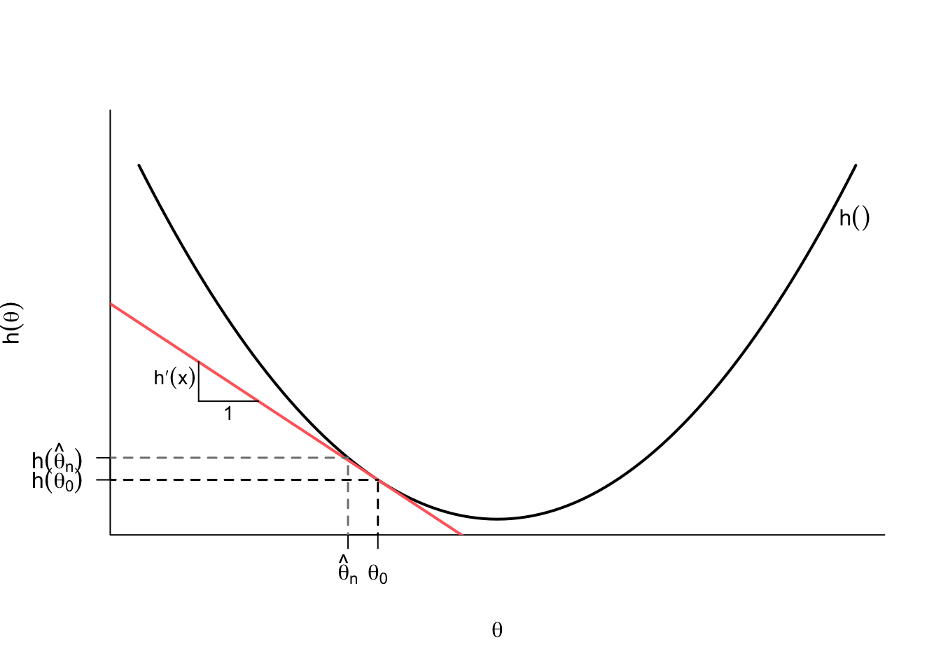
Understanding what’s happening here is useful since it might help give intuition as to when this might go wrong. Why do we focus on continuously differentiable functions, \(h()\)? These functions can be well-approximated with a line in a neighborhood around a given point like \(\theta\). In Figure 3.5, we show this where the tangent line at \(\theta_0\), which has slope \(h'(\theta_0)\), is very similar to \(h(\theta)\) for values close to \(\theta_0\). Because of this, we can approximate the difference between \(h(\widehat{\theta}_n)\) and \(h(\theta_0)\) with the what this tangent line would give us: \[ \underbrace{\left(h(\widehat{\theta_n}) - h(\theta_0)\right)}_{\text{change in } y} \approx \underbrace{h'(\theta_0)}_{\text{slope}} \underbrace{\left(\widehat{\theta}_n - \theta_0\right)}_{\text{change in } x}, \] and then multiplying both sides by the \(\sqrt{n}\) gives \[ \sqrt{n}\left(h(\widehat{\theta_n}) - h(\theta_0)\right) \approx h'(\theta_0)\sqrt{n}\left(\widehat{\theta}_n - \theta_0\right). \] The right-hand side of this approximation converges to \(h'(\theta_0)Z\), where \(Z\) is a random variable with \(\N(0, V)\). The variance of this quantity will be \[ \V[h'(\theta_0)Z] = (h'(\theta_0))^2\V[Z] = (h'(\theta_0))^2V, \] by the properties of variances.
Example 3.6 Let’s return to the iid sample \(X_1, \ldots, X_n\) with mean \(\mu = \E[X_i]\) and variance \(\sigma^2 = \V[X_i]\). From the CLT, we know that \(\sqrt{n}(\Xbar_n - \mu) \indist \N(0, \sigma^2)\). Suppose that we want to estimate \(\log(\mu)\), so we use the plug-in estimator \(\log(\Xbar_n)\) (assuming that \(X_i > 0\) for all \(i\) so that we can take the log). What is the asymptotic distribution of this estimator? This is a situation where \(\widehat{\theta}_n = \Xbar_n\) and \(h(\mu) = \log(\mu)\). From basic calculus, we know that \[ h'(\mu) = \frac{\partial \log(\mu)}{\partial \mu} = \frac{1}{\mu}, \] so applying the delta method, we can determine that \[ \sqrt{n}\left(\log(\Xbar_n) - \log(\mu)\right) \indist \N\left(0,\frac{\sigma^2}{\mu^2} \right). \]
Example 3.7 What about estimating the \(\exp(\mu)\) with \(\exp(\Xbar_n)\)? Recall that \[ h'(\mu) = \frac{\partial \exp(\mu)}{\partial \mu} = \exp(\mu) \] so applying the delta method, we have \[ \sqrt{n}\left(\exp(\Xbar_n) - \exp(\mu)\right) \indist \N(0, \exp(2\mu)\sigma^2), \] since \(\exp(\mu)^2 = \exp(2\mu)\).
Like all of the results in this chapter, there is a multivariate version of the delta method that is incredibly useful in practical applications. We often will combine two different estimators (or two different estimated parameters) to estimate another quantity. We now let \(\mb{h}(\mb{\theta}) = (h_1(\mb{\theta}), \ldots, h_m(\mb{\theta}))\) map from \(\mathbb{R}^k \to \mathbb{R}^m\) and be continuously differentiable (we make the function bold since it returns an \(m\)-dimensional vector). It will help us to use more compact matrix notation if we introduce a \(m \times k\) Jacobian matrix of all partial derivatives \[ \mb{H}(\mb{\theta}) = \mb{\nabla}_{\mb{\theta}}\mb{h}(\mb{\theta}) = \begin{pmatrix} \frac{\partial h_1(\mb{\theta})}{\partial \theta_1} & \frac{\partial h_1(\mb{\theta})}{\partial \theta_2} & \cdots & \frac{\partial h_1(\mb{\theta})}{\partial \theta_k} \\ \frac{\partial h_2(\mb{\theta})}{\partial \theta_1} & \frac{\partial h_2(\mb{\theta})}{\partial \theta_2} & \cdots & \frac{\partial h_2(\mb{\theta})}{\partial \theta_k} \\ \vdots & \vdots & \ddots & \vdots \\ \frac{\partial h_m(\mb{\theta})}{\partial \theta_1} & \frac{\partial h_m(\mb{\theta})}{\partial \theta_2} & \cdots & \frac{\partial h_m(\mb{\theta})}{\partial \theta_k} \end{pmatrix}, \] which we can use to generate the equivalent multivariate linear approximation \[ \left(\mb{h}(\widehat{\mb{\theta}}_n) - \mb{h}(\mb{\theta}_0)\right) \approx \mb{H}(\mb{\theta}_0)'\left(\widehat{\mb{\theta}}_n - \mb{\theta}_0\right). \] We can use this fact to derive the multivariate delta method.
Theorem 3.12 Suppose that \(\sqrt{n}\left(\widehat{\mb{\theta}}_n - \mb{\theta}_0 \right) \indist \N(0, \mb{\Sigma})\), then for any function \(\mb{h}\) that is continuously differentiable in a neighborhood of \(\mb{\theta}_0\), we have \[ \sqrt{n}\left(\mb{h}(\widehat{\mb{\theta}}_n) - \mb{h}(\mb{\theta}_0) \right) \indist \N(0, \mb{H}\mb{\Sigma}\mb{H}'), \] where \(\mb{H} = \mb{H}(\mb{\theta}_0)\).
This result follows from the approximation above plus rules about variances of random vectors. Remember that for any compatible matrix of constants, \(\mb{A}\), we have \(\V[\mb{A}'\mb{Z}] = \mb{A}\V[\mb{Z}]\mb{A}'\). You can see that the matrix of constants appears twice here, like the matrix version of the “squaring the constant” rule for variance.
The delta method is handy for generating closed-form approximations for asymptotic standard errors, but the math is often quite complex for even simple estimators. It is usually more straightforward for applied researchers to use computational tools like the bootstrap to approximate the standard errors we need. The bootstrap has the trade-off of taking more computational time to implement than the delta method. Still, it is more easily adaptable across different estimators and domains with little human thinking time.